QUERY Function in Google Sheets: Simplifying Data Analysis for Everyday Tasks

Introduction

In our fast data-driven digital landscape, the ability to efficiently analyze and manipulate data is paramount. Whether you're a business professional, a student, or simply someone who deals with spreadsheets regularly, finding ways to streamline your data operations can save you valuable time and effort. That's where the QUERY function in Google Sheets comes into play.

The QUERY function is a versatile and powerful tool that allows you to extract, filter, and sort data based on specific criteria. It enables you to transform raw data into meaningful insights, empowering you to make informed decisions and uncover valuable patterns and trends. By leveraging the QUERY function, you can cut through the clutter of large datasets and extract precisely the information you need.

Syntax and basic usage

The QUERY function in Google Sheets follows a specific syntax that allows you to specify cell ranges and define the query itself using a language similar to SQL (Structured Query Language). Let's break down the syntax and explore some basic usage examples.

The basic syntax of the QUERY function is as follows:

=QUERY(range, query, [headers])

• range: range of cells from which you want to retrieve data. It can be specified using A1 notation (e.g., A1:B10) or a named range.
• ‍query: actual query you want to perform on the range of cells. It consists of the query language that determines how the data will be filtered, sorted, and manipulated.
• ‍headers (optional): by default, the first row of your range is considered as headers. You can set this parameter to 0 if your data doesn't have headers, or to 1 if you want to treat the first row as a header.

When constructing your query, it's important to note that the clauses should be written in a specific order: SELECT, WHERE, GROUP BY, ORDER BY.

• ‍SELECT: This clause is used to specify the columns or expressions you want to retrieve from the data. It is usually the first clause in your query.‍
• WHERE: This clause allows you to filter the rows based on specific conditions. It helps you narrow down the data based on your criteria. You can use comparison operators (e.g., >, <, =) and logical operators (e.g., AND, OR) to define the conditions.
• ‍GROUP BY: This clause is used to group rows together based on one or more columns. It is often used in conjunction with aggregate functions like SUM, COUNT, AVG, etc. to perform calculations on the grouped data.
• ‍ORDER BY: This clause is used to sort the data based on one or more columns in ascending (ASC) or descending (DESC) order.

‍

Basic usage examples

Let's examine some basic usage examples to understand how the QUERY function works:

‍Example 1: Selecting Columns 

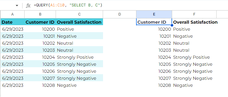
Suppose you have a spreadsheet with data in columns A, B, and C, and you want to select only the data from columns A and C. You can use the QUERY function as follows:

=QUERY(A1:C10, "SELECT B, C")

This query selects columns A and C from the range A1:C10.

Example 2: Filtering Rows 

Imagine you have a dataset with customer data, and you want to filter the rows based on a specific condition, such as displaying only customers with  ‘neutral’ satisfaction. You can use the QUERY function with a WHERE clause:

=QUERY(A1:D10, "SELECT * WHERE C = 'Neutral'")

This query selects all columns (*) and filters the rows to only include those with a value in column C equal to ‘Neutral’.

Example 3: Sorting Data

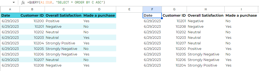
Sorting data is a common requirement when analyzing information. Let's say you want to sort your data in ascending order based on column B. You can use the QUERY function with an ORDER BY clause:

=QUERY(A1:D10, "SELECT * ORDER BY C ASC")

This query selects all columns (*) and sorts the data based on column C in ascending order (ASC).

These examples demonstrate the basic usage of the QUERY function in Google Sheets. Remember the order in which you write the query clauses: SELECT, WHERE, GROUP BY, ORDER

Advanced usage examples

Example 4: Using Joins

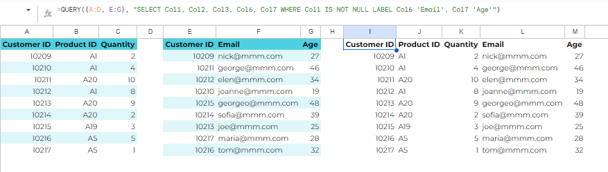
If you have multiple datasets with related information, you can use the QUERY function to perform joins and combine the data. Let's say you have two datasets: one with purchase history (Customer ID, Product ID, Quantity) and another with customer information (Customer ID, Email, Age). You can use a join operation to retrieve the customer information along with their purchase history:

=QUERY({A:D, E:G}, "SELECT Col1, Col2, Col3, Col6, Col7 WHERE Col1 IS NOT NULL LABEL Col6 'Email', Col7 'Age'") 

In this formula, {A:D; E:G} combines the two tables. The QUERY function then selects the desired columns (Customer ID, Product ID, Quantity, Email, and Age) and filters out the empty rows.

‍Example 5: Using Regular Expressions

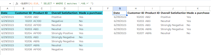
Regular expressions can be powerful tools for pattern matching and extracting specific data. Let's say you have a dataset with product codes, and you want to retrieve all the products with codes that start with "ABC." You can use the QUERY function with regular expressions using the matches operator (~):

=QUERY(A1:E10, " SELECT * WHERE C matches '.*AB.*' ")

In this formula, the QUERY function is used to filter the rows in the range A1:E10 based on a condition specified in the WHERE clause.

The MATCHES operator is used in the WHERE clause to perform a regular expression match. The regular expression pattern used is .*AB.*, where:

The regular expression pattern .*AB.* ensures that the rows in column C containing the substring "AB" anywhere within the text will be selected.

Example 6: Combining Multiple Conditions with Logical Operators

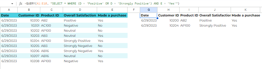
Imagine you have a dataset of customer feedback, and you want to filter the rows based on multiple conditions. Specifically, you want to display the feedback from customers who rated the product as either "Positive" or "Strongly Positive" and made a purchase. You can use the QUERY function with logical operators (OR and AND) to achieve this:

=QUERY(A1:E10, "SELECT * WHERE (D = 'Positive' OR D = 'Strongly Positive') AND E = 'Yes'")

In this formula, the QUERY function selects all columns (*) and filters the rows based on the following conditions:

• The value in column D should be either "Positive" or "Strongly Positive" (using the OR operator).
• The value in column E should be "Yes" (using the AND operator).

By combining multiple conditions using logical operators, you can precisely filter your data based on complex criteria.

Conclusion 

To summarize, the QUERY function in Google Sheets is a powerful tool for efficient data analysis and manipulation. It allows you to extract, filter, and sort data based on specific criteria, transforming raw data into meaningful insights. Whether you need to select specific columns, filter rows based on conditions, perform joins between multiple datasets, or use regular expressions for pattern matching, the QUERY function empowers you to streamline your data operations and make informed decisions. Embrace this powerful tool, and witness your data-driven journey ascend to new heights of efficiency and strategic brilliance.